Interpolation of Lidar Point Clouds
对不同网格大小的精度评估
代表地形高度激发的aimed at creating an EU spatial data infrastructure, has developed specifications for digital terrain models (DTMs). DTMs are preferred as the main source for computing risks of flooding and other analytical tasks while their quality should be specified in terms of accuracy and resolution, i.e. grid size. Here, the author applies five interpolation methods to two airborne Lidar datasets both located in northwest Italy – one capturing a mountainous area and the other a flat urban area – and investigates the resulting accuracy for diverse grid sizes.
Interpolation Methods
The five interpolation methods used are: inverse distance weighting (IDW), natural neighbour (NN) and three variations on splines. In both the IDW and NN methods, heights of unknown points are calculated as a weighted average of known points in the vicinity. In IDW the influence of known points depends on a power of the distance to the unknown point. Other setting parameters are the number of known points and the size and shape of the search area. The power was set to 2, the radius to variable and the maximum number of points to 12. NN uses area derived from a Voronoi tessellation to define the weight. No parameters have to be specified. The third, fourth and fifth methods are based on splines. This approach is well suited for the creation of smoothly varying surfaces. The three variations on splines are: regularised (SpR), tension (SpT), and tension with barriers (SpTb). Breaklines may be included in SpTb by defining weight and number of points. For the regularised method, the weight defines the smoothness of the surface; the higher the weight, the smoother the surface. Typical values are 0, 0.001, 0.01, 0.1 and 0.5. In this study, 0.1 was used. In the tension method: the higher the weight, the coarser the surface. Typical values are 0, 1, 5, and 10. In this case, 0.1 was used. The more points, the smoother the surface will be at the expense of longer computation times. Here, the same number of points was used as for IDW, namely 12. Kriging has been excluded as the results would be similar to splines.
Test data and area
The test data, which was captured over two areas in Italy – Bardonecchia and Grugliasco (Figure 1) – has been acquired through airborne Lidar using the Leica Geosystems AL S50-II. This system employs multiple pulses in air (MPiA), has a maximum pulse rate of 150kHz and a scanning frequency of 90 lines per second while it records 4 returns, including first and last. The survey was originally aimed at creating orthoimagery at scale 1:5,000 and bare ground DTMs with height accuracy (combined systematic and random error) of 0.6m and a grid size of 5m. The actual survey was conducted with a pulse rate of 66.4kHz and scanning frequency of 21.4Hz while the intensities of the four returns were recorded. Points reflected on vegetation and buildings were removed using filters. Table 1 shows other key survey parameters.
Flying height |
200m-6,000m above ground |
视野(FOV) |
58º |
平均点密度 |
0.22分/平方米 |
平均点间距 |
2.12 pts/m |
桌子1, Lidar survey specifications.
尽管大小相似,但两个测试区域的地形特征差异很大。Bardonecchia位于西阿尔卑斯山,靠近法国边界,覆盖39.20公里的面积为39.20公里,高度从1,230m到2,200m不等。Grugliasco是一个位于都灵以西10公里的市区,覆盖38.44km²,高度从260m到470m不等,因此相对平坦。Bardonecchia遗址和近1100万个Grugliasco地点捕获了超过1200万个激光雷达点,鉴于该地区 - 平均密度分别为每3.26m²1分和每3.54平方米1分。使用摄影测量工作站从立体声图像中手动提取了通过SPTB进行插值所需的断裂线。
Results
As the aim was to quantify how interpolation diminishes the accuracy with respect to the original Lidar points, around 1% of the Lidar points were randomly selected as check points. The other 99% were iteratively resampled to generate eight subsets with subsequent lower densities (Table 2). Each subset was interpolated with the five methods described above at three grid sizes: 5 x 5m, 10 x 10m and 20 x 20m. Next each grid height was compared with the height at the check point. To determine the height at the exact corresponding location, bilinear interpolation was applied using four surrounding check points. The root mean square error (RMSE) was computed using Esri ArcGis 10.1 and Python scripting. Residuals and statistical analyses were executed using the free software environment for statistical computing and graphics of the R project (http://www.r-project.org/)。
密度 [1 pnt per ] |
Bardonecchia |
Grugliasco |
|
1 |
3.54m² |
11,897,765 |
10,855,704 |
2 |
5m² |
7,841,600 |
7,687,680 |
3 |
10m² |
3,920,800 |
3,843,840 |
4 |
20m² |
1,960,400 |
1,921,920 |
5 |
50m² |
784,160 |
768,768 |
6 |
100m² |
392,080 |
384,384 |
7 |
200m² |
196040年 |
192,192 |
8 |
400平方米 |
98,020 |
96,096 |
桌子2,八个子集由迭代地重采样到Courser密度。
Bardonecchia的每种方法的结果24 RMS示于图2所示,图3中的Grugliasco中显示了。请注意,水平轴上的0表示原始点密度。Grugliasco(平坦的城市地区)的RMS是比Bardonecchia的数量级要高3至4。IDW和NN成功地生成了所有8个子集的网格。花键无法应对每10平方米最多1点的密度数据集,甚至会产生峰值。图形的锯齿状形状清楚地表明,可以预期的是,准确性随着点密度降低而降低,即RMSE变大,IDW受到最大影响(粉红色线)。随着电网尺寸的增加,所有方法的准确性迅速降低,而对于城市区域(Grugliasco)而言,这种影响比山区(Bardonecchia)更为严重。
Acknowledgements
Thanks are due to Gianni Siletto for providing the airborne Lidar data.
进一步阅读
贝特C·W。合作社。(2009) Evaluating error associated with Lidar-derived DEM interpolation,计算机与地球科学, 35:2, pp. 289-300.
Godone D.,Garnero G.(2013)形态参数在数字地形模型插值准确性中的作用:案例研究,欧洲遥感杂志, 46:1, pp. 198-214.
Guarnieri A., Vettore A., Pirotti F., Menenti M., Marani M. (2009) Retrieval of small-relief marsh morphology from terrestrial laser scanner, optimal spatial filtering, and laser return intensity,地貌学,113: 1–2, pp. 12-20.
Guo Q.,Li W.,Yu H.,Alvarez O.(2010)地形变异性和LIDAR抽样密度对几种DEM插值方法的影响,摄影测量工程和遥感, 76:6, pp. 701 – 712.
Lemmens,M。(2014)点云(1) - 处理软件的功能,188金宝搏特邀, 28:6, pp. 16-21.
Gabriele Garnero是都灵大学的地理学教授和意大利都灵理工学院的计划科学教授。他的研究兴趣包括GNSS,摄影测量和遥感的应用;建筑调查;数字制图,GIS和增长性应用程序。
gabriele.garnero@unito.it
Make your inbox more interesting.添加一些地理。
Keep abreast of news, developments and technological advancement in the geomatics industry.
免费注册